Sampling sparse Gaussian Markov Random Fields in R with the Matrix package
Over the past few months I’ve been involved in a fun project with Andrew Zammit Mangion and Noel Cressie at the University of Wollongong. This project involves inference over a large spatial field using a model with a latent space distributed as a multivariate Gaussian with a large and sparse precision matrix (it also involves me learning a lot from Andrew and Noel!). This is my first time working with sparse precision matrices, so I’ve been discovering many new things: what working in precision-space rather than covariance-space means, and how to draw samples from such models even when the number of data points is large. In this post I share a little of what I’ve learned, along with R code. A lot of what follows is derived from the excellent book on this topic by Rue and Held.
Let’s write
\[\tilde{y} \sim N(\tilde{\mu}, Q^{-1}),\]where \(\tilde{y}\) and \(\tilde{\mu}\) are \(n\) element column vectors, and \(Q\) is a sparse \(n \times n\) precision matrix. The \(ij\)th entry of \(Q\), \(Q_{ij}\), has a simple interpretation:
\[\mathrm{cor}(y_i, y_j \mid \tilde{y}_{-ij}) = -\frac{Q_{ij}}{\sqrt{Q_{ii} Q_{jj}}},\]that is, the correlation between \(y_i\) and \(y_j\), conditional on all the other entries in \(\tilde{y}\), is in proportion to the \(ij\)th entry of the precision matrix. Then, if \(Q_{ij} = 0\), \(y_i\) and \(y_j\) are independent given all other entries, and the converse is also true. This is what leads to the interpretation of these systems as Gaussian Markov Random Fields (GMRFs): the ‘Gaussian’ part is (hopefully) obvious, while the ‘MRF’ part arises by constructing a graphical model with nodes labelled from 1 to \(n\), interpreting the non-zero entries \(Q_{ij}\) as indicating that an edge exists between nodes \(i\) and \(j\) (so they are neighbours), and noting that, conditional on its neighbours, a node is independent of its non-neighbours - the Markov property.
A really simple example of a model that can be cast this way is an AR(1) process, where \(y_t = \rho y_{t - 1} + \epsilon_t\), with \(\epsilon_t\) i.i.d. standard normal. For this model, the conditional correlations are \(\rho\) for adjacent entries and zero otherwise. The precision matrix is
\[Q = \begin{pmatrix} 1 & -\rho & & & & \\ -\rho & 1 + \rho^2 & -\rho & & & \\ & -\rho & 1 + \rho^2 & -\rho & & \\ & & \ddots & \ddots & \ddots & \\ & & & -\rho & 1 + \rho^2 & -\rho \\ & & & & -\rho & 1 \end{pmatrix},\]which is very sparse for large \(n\). The covariance matrix, by constrast, is not at all sparse.
So that’s the interpretation of \(Q\), and one reason why working in precision space is valuable. How to sample \(\tilde{y}\)? The usual way, the one I was taught by my PhD supervisor, is to construct the Cholesky decomposition, \(Q = L L^T\), draw \(\tilde{z} \sim N(0, I_n)\), and then set \(\tilde{y} = \tilde{\mu} + L^{-T} \tilde{z}\). This works, because, as Wikipedia tells us, an affine transformation \(\tilde{c} + B\tilde{x}\) with \(\tilde{x} \sim N(\tilde{a}, \Sigma)\) has distribution \(N(\tilde{c} + B\tilde{a}, B \Sigma B^T)\), and in our case this means that \(\tilde{y}\) has mean \(\tilde{\mu}\), and covariance
\[L^{-T} I_n L^{-1} = L^{-T} L^{-1} = (LL^T)^{-1} = Q^{-1}\text{.}\]It turns out that there are Cholesky decomposition algorithms that are efficient for sparse matrices, but there is a catch. Consider the following sparse 100x100 precision matrix with just 442 non-zero entries:
library(Matrix)

str(Q_100)
## Formal class 'dsCMatrix' [package "Matrix"] with 7 slots
##   ..@ i       : int [1:442] 0 1 0 2 3 4 3 5 5 6 ...
##   ..@ p       : int [1:101] 0 1 2 4 5 6 8 10 11 14 ...
##   ..@ Dim     : int [1:2] 100 100
##   ..@ Dimnames:List of 2
##   .. ..$ : NULL
##   .. ..$ : NULL
##   ..@ x       : num [1:442] 8 8 -0.96 8 5 ...
##   ..@ uplo    : chr "U"
##   ..@ factors : list()
where the length of the @i entry gives the number of non-zero values. Here I am using the Matrix package, which is very well engineered and has tons of useful sparse matrix classes and functions. We can use image to visualise the sparsity pattern:
image(Q_100)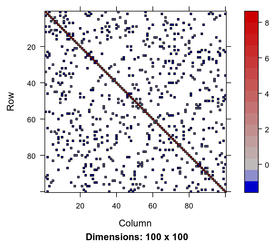
The direct Cholesky decomposition of this matrix is
chol_Q_100 <- t(chol(Q_100))

str(chol_Q_100)
## Formal class 'dtCMatrix' [package "Matrix"] with 7 slots
##   ..@ i       : int [1:2403] 0 2 8 11 24 33 40 55 91 1 ...
##   ..@ p       : int [1:101] 0 9 18 29 35 44 51 62 71 84 ...
##   ..@ Dim     : int [1:2] 100 100
##   ..@ Dimnames:List of 2
##   .. ..$ : NULL
##   .. ..$ : NULL
##   ..@ x       : num [1:2403] 2.828 -0.339 -0.339 -0.339 -0.339 ...
##   ..@ uplo    : chr "L"
##   ..@ diag    : chr "N"

image(chol_Q_100)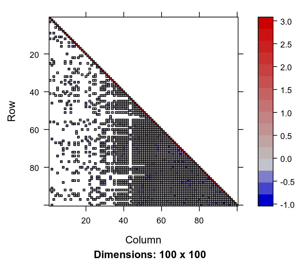
which has 2403 non-zero entries, around 6 times less sparse the original matrix. In general there is no guarantee that the Cholesky decomposition of a sparse matrix will be particularly sparse.
However, all is not lost. If one permutes the indices of \(\tilde{y}\), the precision matrix of the permuted vector is just \(Q\) with rows and columns permuted the same way. It turns out that this can often be done in such a way that the Cholesky decomposition of the permuted precision matrix is much sparser than that of the original matrix. Algorithms that find these permutations are called minimum degree algorithms, but the problem in general is NP-hard, so that finding an optimal permutation is infeasible. Still, fast approximate algorithms exist and work well, and are also available in the Matrix package:
chol_Q_100_permuted <- Cholesky(Q_100, LDL = FALSE, perm = TRUE)
str(chol_Q_100_permuted)
## Formal class 'dCHMsimpl' [package "Matrix"] with 10 slots
##   ..@ x       : num [1:932] 1.732 -0.268 -0.339 -0.268 2.22 ...
##   ..@ p       : int [1:101] 0 4 9 15 21 29 38 46 54 62 ...
##   ..@ i       : int [1:932] 0 1 5 6 1 2 5 6 7 2 ...
##   ..@ nz      : int [1:100] 4 5 6 6 8 9 8 8 8 6 ...
##   ..@ nxt     : int [1:102] 1 2 3 4 5 6 7 8 9 10 ...
##   ..@ prv     : int [1:102] 101 0 1 2 3 4 5 6 7 8 ...
##   ..@ colcount: int [1:100] 4 5 6 6 8 9 8 8 8 6 ...
##   ..@ perm    : int [1:100] 78 97 62 53 85 51 83 43 25 52 ...
##   ..@ type    : int [1:4] 2 1 0 1
##   ..@ Dim     : int [1:2] 100 100

P <- as(chol_Q_100_permuted, 'pMatrix')
image(P %*% Q_100 %*% t(P), main = 'Q (permuted)')
image(chol_Q_100_permuted, main = 'Cholesky')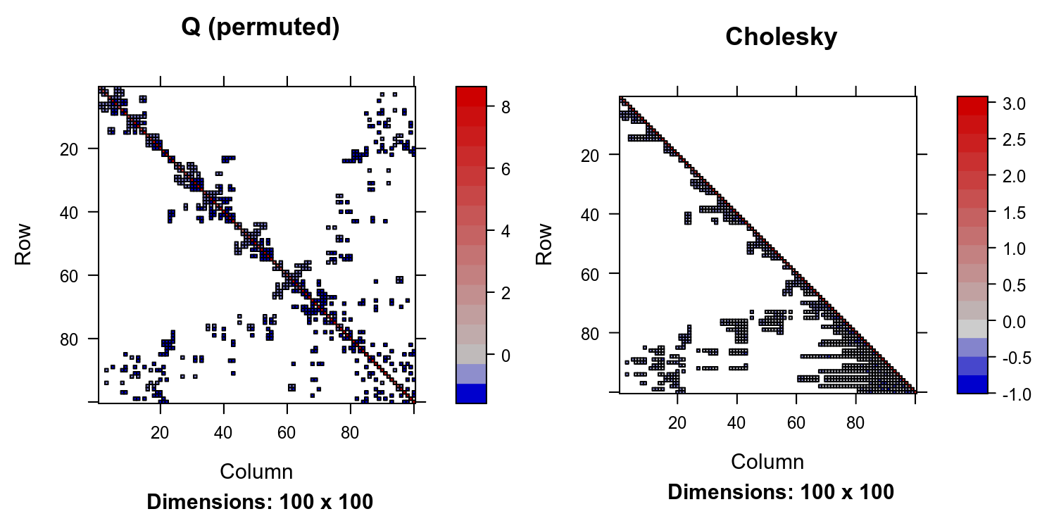
The Cholesky of the permuted system is only twice as dense as the precision matrix, with 932 non-zero entries versus 442 in \(Q\). Mathematically, this permuted decomposition can be written as
\[Q = P^T L L^T P\text{,}\]where \(P\) is a permutation matrix (for which, handily, \(P^{-1} = P^T\)). A simple rearrangement gives \( L L^T = P Q P^T \), showing that \(L\) factorises the permuted \(Q\). In the implementation in the Cholesky function in the Matrix package, the matrix \(P\) is found using heuristics in the CHOLMOD library, which seem to do a good job most of the time. Now, finally, returning to the problem of sampling using a sparse precision matrix, we can again draw \(\tilde{z} \sim N(0, I_n)\), and then set \(\tilde{y} = \mu + P^T L^{-T} \tilde{z}\), which works because the resulting samples have the covariance matrix
exactly as desired. In R this can be implemented (assuming \(\tilde{\mu} = 0\)) as
z <- rnorm(nrow(Q_100))
y <- as.vector(solve(chol_Q_100_permuted, solve(chol_Q_100_permuted,
  z,
  system = 'Lt'
), system = 'Pt'))

print(y)
##   [1] -0.010436811 -0.104921003  0.416806878  0.014558426 -0.325958512  0.421416694
##   [7]  0.017556657  0.294846807  0.342143599  0.584348518 -0.745948125  0.502591827
##  [13] -0.211289349 -0.530267664 -0.492578588  0.255440512 -0.033373118  0.543754332
##  [19] -0.359336565 -0.244953719 -0.402822998  0.081855516  0.253129386  0.205448992
##  [25]  0.429277080 -0.570717950 -0.355061101 -0.367764418  0.547808516  0.006163957
##  [31]  0.547535317  0.263772641  0.081585252  0.358314917 -0.684981518  0.349907450
##  [37]  0.118787977  0.736998466  0.291061633  1.014721231 -0.654090497  0.076018863
##  [43] -0.242907011 -0.535462456 -0.604620123  0.067914043  0.794672200  0.012960978
##  [49]  0.760320360 -0.624262194 -0.009172130  0.125357591  0.708511268 -0.256838400
##  [55]  1.230920479 -0.025501688 -0.282647795 -0.516675265 -0.156191890 -0.030417522
##  [61] -0.778278611 -0.625331836  0.452920865  0.131189388 -0.380328115  0.390079796
##  [67] -0.076916683 -1.042158717  0.243373908 -0.364218763  0.440914464 -0.099416308
##  [73]  0.353931288 -0.197764896  0.289573501 -0.340746684  0.126392280  0.645720329
##  [79]  0.307557118  0.135445659  0.358892563  0.275572959  0.221368375  0.800978241
##  [85] -0.306959557  0.111877324 -0.245831320  0.281856754 -0.183687867 -0.132821530
##  [91] -0.241247800  0.068393000 -0.089732671 -0.191843241 -0.313567706 -0.186392786
##  [97]  0.656691494 -0.083198611 -0.160093445  0.377602280
and the sample can be visualised as
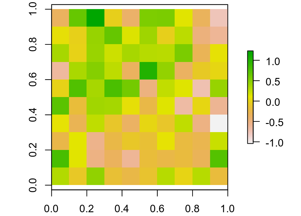
which shows a fair amount of correlated structure (at least it does to me).
As a programming aside, the chol_Q_100_permuted object produced by the Cholesky function is an S4 object of class CHMfactor that contains both the permutation matrix \(P\) and the decomposition \(L\). You can extract these like so:
P <- as(chol_Q_100_permuted, 'pMatrix')
L <- as(chol_Q_100_permuted, 'Matrix')
and manipulate them directly, but it’s generally more efficient to use the solve method associated with the CHMfactor class:
# Calculates solve(Q_100, b), the solution to the original matrix system:
solve(chol_Q_100_permuted, b, system = 'A')
# Calculates L %*% b:
solve(chol_Q_100_permuted, b, system = 'L')
# Calculates t(L) %*% b:
solve(chol_Q_100_permuted, b, system = 'Lt')
# Calculates P %*% b:
solve(chol_Q_100_permuted, b, system = 'P')
# Calculates t(P) %*% b:
solve(chol_Q_100_permuted, b, system = 'Pt')
These use fast CHOLMOD routines that are generally faster than extracting the raw internals, and as a bonus they avoid the extra copying associated with that extraction.